Evidence for the first globular cluster stellar stream beyond the Milky Way

Recent capabilities to detect low-surface-brightness objects have led to the discovery of numerous UDGs^13,14: galaxies with dwarf-like stellar masses but MW-like extents¹⁵. The methods available for inferring their detailed mass and density distribution remain limited, as their characteristic low surface brightness means that measuring velocity dispersions or rotation curves is challenging¹⁶.

Figure 1 shows observations of the UDG UGC 9050-Dw1 by the HST and the Canada–France–Hawaii Telescope (CFHT), in which we highlight a feature resembling one arm of a stellar stream extending from a GC candidate. The thin stream candidate and its presumed parent GC have a projected distance of about 2.5 kpc to the centre of UGC 9050-Dw1, which is probably associated with the low-surface-brightness spiral galaxy UGC 9050 at a distance of 35.2 ± 2.5 Mpc (refs. ^17,18). UGC 9050-Dw1 was first identified in CFHT images as part of a diffuse dwarf galaxy search¹⁹. The HST image was presented in a detailed analysis of UGC 9050-Dw1’s GC population, which found that most of the GCs probably formed simultaneously during a past dwarf merger event¹⁷. The stream-like feature, which we name Oyashio (after a cold Pacific ocean current, pronounced [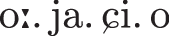], inspired by the nomenclature introduced in ref. ²⁰), is identified independently in the HST and CFHT data, ruling out imaging or data processing artefacts as its origin. All available data are shown in Extended Data Fig. 1.

A comparison between the background-subtracted image counts, f, of the stream candidate and the standard deviation of the background, σ, gives a signal prominence of \(({f}_{{\rm{stream}}}-\,{\overline{f}}_{{\rm{background}}})/{\sigma }_{{\rm{background}}}=7.34\) in the combined HST image. We measure the width of the stream candidate to be w_±σ = 72.3 ± 8.9 pc, assuming a Gaussian profile (see Methods and Extended Data Fig. 2). The amplitude, A, of this fit gives a signal-to-noise ratio of \(A/\sqrt{{\sigma }_{A}}=5.2\) for the HST image and similar fits to the CFHT images give ratios ranging between 2.3 and 3.9 in all g-band, r-band and i-band images, whereas the feature is not detectable in the u and z bands.

GC streams in the MW have widths ranging from a few tens to a few hundred pc (ref. ²¹). The width of Oyashio is much smaller than any known stream from a dwarf galaxy progenitor (for example, the Orphan–Chenab MW stream, which has a low-mass dwarf progenitor but a width >200 pc (ref. ²²)), pointing towards a GC origin. The length of the Oyashio stream arm is 2 kpc based on a by-eye estimate.

The stellar population of a GC progenitor and its stream are of the same age and metallicity and therefore follow the same track (isochrone) in a colour-magnitude diagram. In the MW, these tracks can be analysed at the level of individually resolved stars. At the distance of UGC 9050-Dw1, we must consider the integrated-light equivalent: comparing the overall colour of the stream and progenitor. Many of the GC candidates in UGC 9050-Dw1 have similar colours, probably because of simultaneous formation¹⁷, so we also expect this particular GC candidate and its stream to align with the colours of the other GCs in the host. In Fig. 2, we show that the Oyashio stream and progenitor cluster candidates have overlapping colours, as expected if they share the same stellar population, and both fall within the GC candidate selection box used in ref. ¹⁷. The GC candidate has a colour of F555W-F814W = 1.1 ± 0.1 and the stream-like feature has F555W-F814W = 1.0 ± 0.2. This is slightly bluer than the average GC in the MW (refs. ^23,24), which aligns with the findings in ref. ¹⁷ that the clusters in UGC 9050-Dw1 are consistent with a more recent origin.

To test whether a GC stream with this morphology at this location is dynamically plausible, we apply the X-Stream sampler⁶, which translates stream imaging into constraints on stream progenitors and host dark matter halos. See Methods and Extended Data Table 1 for details on the model parameters. In Fig. 3a, we show the likelihood surfaces and sampler constraints on the progenitor mass, halo mass and on the inner density slope of the halo, γ, from the sampler applied to control points generated within a mask of width w_±2σ = 143.7 pc. The orange contours show the 68% and 95% credible regions for runs with a dark matter halo concentration of c = 5 and the grey contours show the same regions for the c = 2 runs.

We treat these c = 5 runs as our fiducial runs (see posteriors in Extended Data Table 1), as varying the mask width or concentration does not make a material difference in our results, which we discuss in Methods.

For our fiducial runs, the sampler places an upper limit on the initial progenitor mass of M_p < 2.5 × 10⁶ M_⊙ with 95% confidence. These mass constraints are consistent with our interpretation of a GC origin for the stream²¹ and is less massive than, for example, the MW star cluster Omega Centauri (M_* = 3.55 × 10⁶ M_⊙)²⁵ with its associated stream²⁶ and comparable with some GCs in M31 (ref. ²⁷).

The surface brightness of Oyashio in the HST images is F555W = 27.0 ± 0.1 mag arcsec⁻², F814W = 26.1 ± 0.1 mag arcsec⁻². This is brighter than the average MW stream²⁰, which is to be expected for an extragalactic discovery. We compare the measured surface brightness of the stream candidate to a simulated stellar population based on that of the archetypal MW GC stream Palomar 5 (denoted Pal 5 hereafter)²⁸ and find that a stream with the same age, metallicity and level of disruption requires a progenitor 20 times as massive, that is, an initial cluster mass of about 2 × 10⁶ M_⊙, to produce a similar surface brightness as our detected stream candidate. We repeat this analysis for a grid of isochrones and find that a younger progenitor can produce the observed surface brightness with a progenitor mass as low as 1.65 × 10⁵ M_⊙ for the brightest isochrone, for which we use the brightness ratio between the stream and GC candidates to gauge the level of disruption. We note that the GC population of UGC 9050-Dw1 is relatively blue and consistent with younger GCs than Pal 5 (ref. ¹⁷).

The red dots and stars in Fig. 3a represent the lower bound and 20× Pal 5-like progenitors, respectively. These points are both within the 95% confidence regions of the posteriors.

The X-Stream sampler finds a UGC 9050-Dw1 halo scale mass⁶ of \({\log }_{10}({M}_{{\rm{h}}}/{M}_{\odot })=11.3{1}_{-0.71(-1.30)}^{+0.67(+1.03)}\) within the 68% (95%) confidence limit, which corresponds to \({\log }_{10}({M}_{200}/{M}_{\odot })=11.6{3}_{-0.83}^{+0.71}\) (68%) using Planck cosmological parameters²⁹ and finds \(\gamma =0.9{2}_{-0.58(-0.87)}^{+0.57(+0.92)}\) within the 68% (95%) confidence limits. This is the first constraint on a dark matter halo mass and density slope from a stellar stream in an UDG. It suggests that this UDG is slightly less cored than the average low-surface-brightness dwarf (γ ≈ 0.2) (ref. ³⁰), and UDG Dragonfly 44 (γ = 0.3) (ref. ⁴), but allows inner slopes comparable with that of UDG AGC 242019 (γ ≈ 0.54) (ref. ⁵). The sampler also places strong constraints on the line-of-sight progenitor position and on the progenitor orbit, whereas the halo scale radius and outer density slope are unconstrained. We show the full posterior distributions for the fiducial run in Extended Data Fig. 4. In Extended Data Fig. 5, we show examples of five streams within the 68% confidence regions (good fits) and five outside the 95% region (inconsistent fits). While the good fits reproduce the observed input data well, the inconsistent fits are too straight, too curved, offset from the input data or too wide.

In Fig. 3, we show two streams models: the lower bound stream, selected on the basis of our surface brightness analysis above to have a progenitor mass of 1.65 × 10⁵ M_⊙ (Fig. 3b), and the 20× Pal 5-like stream, selected to have a progenitor mass of 2.00 × 10⁶ M_⊙ (Fig. 3c). All other parameters were selected at random within the 68% credible region of the likelihood surface. Both model streams reproduce the morphology of the observed input data well, but the 20× Pal 5-like stream is longer. We mock-observe these two streams and show the results in Extended Data Fig. 6 (top and middle panels). The densest parts of the mock-observed model streams look similar to the observed stream candidate, whereas the more diffuse end parts of the model streams are not observable. Note that the arm towards positive x-values, which was not included in the fitting procedure, wraps behind the brighter central part of the UDG itself. This can help explain why we only detect one arm in the HST data.

For the model stream in Fig. 3c, for which the halo mass is at the peak of the posterior distribution, the progenitor’s current galactocentric radius is R_gal,today = 2.52 kpc, the inferred enclosed mass of the UDG is M(<R_gal,today) = 1.36 × 10¹⁰ M_⊙. The total mass (M₂₀₀ = 1.56 × 10¹¹ M_⊙) is similar to mass estimates of the Large Magellanic Cloud^31,32 and is within errors of previous halo mass estimates¹⁷, which used the GC count to calculate a total halo mass of 1.5 ± 0.3 × 10¹¹ M_⊙ or 1.8 ± 0.3 × 10¹¹ M_⊙, depending on the assumptions made. The entire mass range of ref. ¹⁷ is within our allowed halo masses for all runs.

The tidal radius, \({r}_{{\rm{t}}}\propto {R}_{{\rm{gal}}}{\left(\frac{{M}_{{\rm{p}}}}{{M}_{{\rm{h}}}}\right)}^{1/3}\), of a GC determines the boundary at which stars become unbound from the progenitor and can escape into the leading and trailing arms of the stream. If r_t is much larger than the extent of the cluster, a stream cannot form (see, for example, ref. ³³). For the fit shown in Fig. 3c, the present-day r_t = 133 pc and the minimum r_t = 95 pc. This is similar to the estimated tidal radius of Pal 5 (≈145 pc) (ref. ³⁴).

Because the cluster with the lower bound progenitor mass (Fig. 3b) is evolving in an even higher mass halo, we conclude that tidal stripping is feasible for both clusters presented in Fig. 3 and that our dynamical models are consistent with a GC being tidally stripped with M_p < 2.5 × 10⁶ M_⊙ at 95% confidence.

There are other mechanisms that could potentially create a similar structure in an image. Recent observations have reported evidence of tidal tails from mergers of GCs or nuclear star clusters in dwarf galaxies³⁵. Tidal tails are formed as a result of mutual interactions between two low-mass-ratio objects rather than from Lagrange point stripping of high-mass-ratio objects, such as a GC and a host galaxy halo, which leads to the formation of stellar streams. In the case of merger-induced tails, we expect them to occur near the host centre. This scenario is unlikely to explain the feature presented in this paper, which has a distance >2 kpc from the luminosity centre of the host UDG. So far, no extragalactic stellar streams from GC progenitors have been confirmed and previous candidates have been shown to be physically implausible^36,37,38 or simply not detected at a statistically significant level above the background stellar halo, even in nearby galaxies such as M31 (ref. ³⁹).

A tidal shell formed in a radial collision between two stellar systems can also appear as a thin curved structure (for example, ref. ⁴⁰). However, the centre of curvature for Oyashio is offset from the centre of the host, which is not expected for shells. Similarly, a lensing effect of a background galaxy could create an arc^41,42, but we do not observe other arcs or any plausible lenses. Furthermore, the stream’s alignment with the GC candidate and the fact that their colours are similar to the other GCs in the system would need to be coincidental. Alternatively, a dusty region may lead to fluctuations mimicking the stream candidate. If there were a dust patch in the region on one side of the stream, we would expect it to be redder than on the other side. We find no evidence of such a trend.

A stellar stream from a small dwarf galaxy might be misinterpreted as a GC stream. In the case presented here, the observational width measurement and the dynamical mass constraints both point to a GC progenitor. We might only be observing the densest part of the stream, but even with a larger mask width, our modelling mass constraints point to a GC origin. In Extended Data Fig. 6 (bottom), we also mock-observe a dwarf-like stellar stream with the same stellar mass as our 20× Pal 5-like stream but including dark matter. The dwarf-like stream has a larger surface area, yielding a lower surface brightness. For the dwarf stream to be observable, it would need an approximately 5× larger stellar mass than our reported upper limit of the progenitor mass and such a stream would be observed as wider than Oyashio in the HST data.

Last, there is the possibility of a chance alignment of unresolved stars in the host galaxy or a chance projection of stars unassociated with the host. Although chance alignment or chance projection cannot be entirely ruled out, the similarity in colours and the agreement between modelling results, halo mass estimates from GC counts and our mock observations support a GC stream detection. It also seems likely that the first extragalactic GC stream to be detected would  reside in a massive halo of a low-surface-brightness galaxy, facilitating tidal stripping while providing a faint background.

Deeper observations with the HST or the James Webb Space Telescope of this object could distinguish it further from background and thus determine its origin with greater certainty. Spectroscopic studies with, for example, the Keck telescope (similar to refs. ^1,43) could compare parts of the Oyashio stream candidate to the presumed parent cluster to reveal similarities and differences in stellar populations.

UGC 9050-Dw1, like many UDGs, has a complex morphology, which is one of the reasons that their dark matter mass and density profiles are not well understood^5,44. Stellar streams from GCs are sensitive to the local acceleration field^8,45 and our results provide the first-of-its-kind UDG mass and density constraints, introducing a new tool to study UDGs.

Cold dark matter models predict the formation of low-mass subhalos devoid of stars⁴⁶ and a detection would put tight constraints on the properties of candidate dark matter particles⁴⁷. A promising avenue for detecting low-mass subhalos is through their interaction with stellar streams¹⁰, which can create variation in the stream density^7,9. Extending the sample of GC stellar streams to include extragalactic hosts, as done in this work, allows us to study host galaxies with fewer baryonic perturbers than the MW, which will increase the chances of an unambiguous subhalo detection⁴⁸.

A GC stellar stream visible at a distance of 35.2 Mpc highlights the potential of discoveries in neighbouring diffuse galaxies, especially if GC streams are as frequent in UDGs as extrapolated MW counts suggest^11,12. With the capabilities of the Euclid and Roman space telescopes^49,50, we expect to detect many more GC streams^37,39,51. The extragalactic GC stellar stream presented in this paper serves as a precursor to future detections and represents an independent way to investigate the dark matter mass and density profiles of UDGs.

Data

The HST Advanced Camera for Surveys (ACS) images use the Wide Field Channel (WFC) in the F555W and F814W filters, have an angular resolution of 0.1″ and reach exposure times of 2,406 s and 2,439 s, respectively. The observations were carried out in September 2022 under HST programme ID 16890 (ref. ⁵²) and the resulting images of UGC 9050-Dw1 were presented in ref. ¹⁷. The images have been calibrated through the standard HST CALACS pipeline and are available on the STScI/MAST archive.

CFHT has observed the same region of the sky using MegaCam as part of its Legacy Survey in 2005 and UGC 9050-Dw1 was first identified and selected in a semi-automated search for diffuse dwarfs¹⁹. The area containing UGC 9050-Dw1 is visible in both the W3-1-3 and W3-2-3 fields of the survey, which contains bands u, g, r, i and z, so a total of ten CFHT images are available. Because of the signal-to-noise levels, we are not able to confidently identify the stream-like feature in the u-band or z-band images. Integration times, observation depth and seeing for the CFHT data are published in ref. ⁵³. The CFHT data, which have been calibrated through the MegaPipe pipeline, are available through the Canadian Astronomy Data Centre.

For visual purposes, we have smoothed the HST and CFHT images using a Gaussian kernel (with σ = 3 and 1.5 pixels, respectively) and we plot the area of interest in all available bands in Extended Data Fig. 1. All data analysis is performed on unsmoothed data.

Data analysis

The feature was initially detected by eye, but when we apply the rolling Hough transform⁵⁴ with a range of (hyper)parameters, the code consistently returns both the location and curvature of the stream candidate. We use this as a validation of the initial by-eye detection.

In Extended Data Fig. 2 (left), we rotate the images into a coordinate frame aligned with the stream, in which (ϕ₁, ϕ₂) represents stream longitude and latitude^55,56. We draw masks around the stream by following a polynomial fit to points selected manually in the F814W image, creating a curved shape with constant width, excluding the GC candidate. We duplicate these on both sides to mask the background areas. To measure the width, we sample slices perpendicular to the track curvature in steps of pixel size along this fit. We collapse the resulting area along the fitted track, calculating the mean brightness of the stream candidate and its surrounding areas. The right panels of Extended Data Fig. 2 depict the perpendicular brightness profile, consisting of the average brightnesses measured parallel to the curved stream track. This is done in six segments to check for any single dominating contaminant. We fit a Gaussian with a linear offset to the perpendicular brightness profile for each segment, as well as the whole stream. This way of sampling the surrounding area causes the inner part of the curve to be oversampled compared with the outer curve and thus, by construction, it has a lower error and dominates the fit. We therefore use the average of all standard deviations as uniform errors. The standard deviation of the Gaussian provides an estimate of the width of the stream, with uncertainties on the fitted parameter. Because σ describes the deviation from the mean, μ, the total width is twice σ. We denote this width, measured from μ − σ to μ + σ, as w_±σ. The width that includes 95% of the Gaussian area, corresponding to 2σ from the mean, we call w_±2σ. The physical width is affected by the instrument point spread function (PSF), which we account for by subtracting the observational dispersion in quadrature. We use the full width at half maximum for HST of 0.1″.

The seeing of the CFHT observation (0.88″) is comparable with the width of the feature in the CFHT images (w_±σ = 1.1″). Therefore, we use the HST width in subsequent analysis.

There is a brighter object located next to the track at around ϕ₁ = −4, which increases the measured width. If we only use the track up to that point, it yields a width of w_±σ = 52 pc instead. On the other hand, the faintness of the object means that we might only be sensitive to the brightest central part of our stream candidate, which would lead to an underestimated width. In Extended Data Fig. 6, we illustrate that the simulated GC streams show up with similar apparent width when injected into the data.

To quantify the prominence of the stream candidate, we sum the counts in the on-stream mask and in the off-stream background masks. We subtract the mean background from the signal and compare this with the standard deviation of the backgrounds: \(({f}_{{\rm{stream}}}-\,{\overline{f}}_{{\rm{background}}})/{\sigma }_{{\rm{background}}}\).

The Gaussian fit used in the width measurement also gives a signal-to-noise ratio when we compare the amplitude to its fit uncertainty, \(A/\sqrt{{\sigma }_{A}}\). This uncertainty takes into account the error on the means, which were included in the fit. Neither prominence estimate includes the GC candidate; they are based only on light from the stream candidate.

The statistical significance contains three main components: the probability that it is a stream, the probability that we would find it and, given that the first two statements are true, the statistical significance of the signal in the data. What we quote as a significance is only the last of these.

To compare the colours of the stream and cluster candidates to other GC candidates in the host UDG, we sum their brightness in each of the two available HST filters. The stream area is defined as a curved shape with the constant width found above (w_±2σ = 16.8 pixels = 143.7 pc) around a polynomial fitted to an array of manually selected points along the track. The cluster is contained in a circular mask 20 pixels (170.6 pc) wide, following a photometric growth-curve analysis similar to, for example, ref. ⁵⁷ to find an aperture radius that includes most of the light. We make sure that the masks of the stream and progenitor do not overlap. Both masks are illustrated in Extended Data Fig. 3 with blue and purple outlines, respectively. All magnitudes are in the Vega system and we correct for galactic extinction using values from ref. ⁵⁸ as calculated through the NASA/IPAC Extragalactic Database (NED) extinction calculator.

For accurate colour measurements, we need to subtract the background of a nearby approximately empty equal area (see, for example, ref. ⁵⁹). Owing to the complex morphology of UGC 9050-Dw1, the choice of this area is not obvious and the resulting colour is greatly affected by the choice. We therefore use the average of several areas distributed on both sides of the stream candidate (illustrated in Extended Data Fig. 3). The errors on the colour values reflect the spread resulting from using either of the background areas on its own, as well as the error on the brightness in each band, which is measured by the standard deviation of pixel values.

The ACS pixel scale of 0.05″ per pixel corresponds to 8.53 pc at this distance. This is comparable with the size expected for GCs (a few pc)⁶⁰ and ref. ¹⁷ therefore treats the GC candidates as point sources. For a partially disrupted cluster, however, we expect a larger physical extent and, by definition, a stream will not resemble a point source. We therefore treat both objects as extended sources, using areas illustrated in Extended Data Fig. 3 as their extent. Our GC candidate is not included in the final GC candidate sample of ref. ¹⁷ and inspection of their selection criteria reveals that it is discarded on the basis of roundness, sharpness and/or magnitude uncertainty. A tidally disrupting GC would be both elongated and more diffuse than the undisturbed clusters, which explains the deviation from all three criteria.

We integrate the light over the areas illustrated in Extended Data Fig. 3 to measure the surface brightness of the stream candidate. This yields a surface brightness of 27.0 ± 0.1 and 26.1 ± 0.1 mag arcsec⁻² in the F555W and F814W filters, respectively, after subtracting the background.

To explore the possible stellar populations in the stream, we use a grid of isochrones with varying age and metallicity. We sample stars from a simple initial mass function (IMF) following \(\frac{{\rm{d}}N}{{\rm{d}}m}\propto {m}^{-0.5}\) (ref. ⁶¹) and truncated on the basis of the mass range of survived stars in each of the isochrones. We extract brightnesses from the interpolated isochrone tracks, generated for HST and CFHT filters through the colour–magnitude diagram input form⁶² using the PARSEC version 1.2S evolutionary model⁶³. We distribute these stars across the area of the stream in the data, including the presumed hidden arm, and we calculate their surface brightness. We decrease the population size until there is only one isochrone that gives a surface brightness comparable with that in the HST data. This population is just visible with the brightest isochrone in our suite and we use its total mass as a lower bound on the possible size of a stream with this surface area producing the observed brightness.

We find that an initial progenitor mass as low as M_⋆,tot = 1.65 × 10⁵ M_⊙, with an 8-Gyr-old stellar population with [M/H] = −1.0, can reproduce the observed surface brightness of the present-day stream.

Because we do not know the detailed mass loss history of the GC candidate, to obtain the total mass of the stream and progenitor, we assume that the brightness ratio between the cluster and stream is an appropriate proxy for the mass ratio. Assuming that the two stream arms are identical, this gives a ratio of M_stream/M_total ≈ 0.75, which we use to scale the inferred stream mass to a total progenitor mass.

For the Pal 5-like stream, we use the same methodology to estimate the level of disruption as in ref. ³⁷. We use an isochrone track with age 11.3 Gyr and metallicity of [M/H] = − 1.3. Pal 5 contains 3,000 stars in the DECAM g band between magnitudes 23 and 20 (ref. ⁵⁹), so we sample the IMF until this threshold is reached and use the resulting sample to calculate the surface brightness of the population. We repeat this process for samples of 5, 10 and 20 times the threshold (corresponding to equal multiplications of Pal 5 mass), the last of which yields a surface brightness matching the values from the HST data. This method assumes a mass loss identical to that of Pal 5.

Generative stream models

To generate stream models, we apply the X-Stream sampler⁶, which uses the particle-spray method⁶⁴ implemented in the GPU code streamsculptor⁶⁵. We fix the escape conditions to those of ref. ⁶⁴. These particle-spray simulations are tuned to reproduce more expensive N-body simulations of GC dissolution. Note that our results are dependent on the stream model escape conditions. We generate streams in a halo potential meant to represent the diffuse dwarf with an inner slope, γ, and outer slope, β (see equation (1) in ref. ⁶). We do not include the baryons in our modelling efforts, as these make up a small fraction of mass compared with the estimated mass of the total system (M_* ≈ 10⁷ M_⊙ within the half-light radius)¹⁷. The dark matter halo profile is thus treated as a representation of the entire diffuse dwarf.

We define the coordinate system in which we generate model streams by transforming the candidate GC progenitor position and the centre of UGC 9050-Dw1 from right ascension and declination to a galactocentric rest frame at which UGC 9050-Dw1 is at the origin using astropy⁵⁶ and the distance to UGC 9050-Dw1 of 35.2 Mpc. x and z define the plane of the sky and y is the line-of-sight direction pointing towards the observer. We fix the on-sky position of the progenitor (x, z) in our models.

In this coordinate system, we outline a mask for the observed stream extending to the left of the candidate GC progenitor. To test how the choice of width affects our results, we use two different mask widths to represent the stream. Our fiducial mask width is w_±2σ = 143.7 pc. We also test a mask width of 185 pc corresponding to w_±3σ. We create a grid of control points within the outlined masks to represent the candidate stream. These control points are used as our input for the X-Stream sampler. Note that we only generate control points for the left side of the stream, as we do not confidently observe a right extension of the stream.

From the control points, we generate a kernel density estimation (KDE). For each model stream, the sampler generates a KDE and uses a Kullback–Leibler divergence test^66,67 to measure the difference between the KDE from each generated model stream and the KDE from the input control points (see details in ref. ⁶). The best-fitting model streams are ones that minimize this difference. Note that particle-spray models do not reproduce the detailed density along the stream but that X-Stream relies on control points and includes an inverse density weighing to smooth over features. Streams wider than the data have excess density inconsistent with the control points and X-Stream thereby disfavours wider models.

We draw a bounding box around the stream mask to ensure that we do not penalize our generated model streams if they are longer than the mask nor if they extend to the right of the progenitor. However, the model streams are penalized if they are shorter than the observed stream.

To sample the parameter space and test which orbits, progenitor properties and halo properties can reproduce the present-day observed candidate stream, we use ten free parameters with uniform, flat priors and fix only the progenitor position in the plane of the sky (Extended Data Table 1). We test two different concentrations for the dark matter halo: c = 2 and c = 5 (as motivated from refs. ^3,5). X-Stream uses a nested sampling technique to examine the large parameter space and the sampler outputs the likelihood of each model stream and the likelihood surface, including the 68% and 95% credible regions for all parameters.

Owing to the known degeneracies for the orbital direction of a stellar stream in the plane of the sky (see Figs. 10 and 8 in refs. ^6,33, respectively), we only sample half of the unit sphere in the velocity space. Thus there are islands of solutions for which the model streams move in the opposite direction (that is, opposite leading and trailing arms), which are equally good fits. However, the distance gradient for such solutions remains the same (see Figs. 10 and 9 in refs. ^6,33, respectively). We list all free and fixed parameters for the X-Stream sampler in Extended Data Table 1. See ref. ⁶ for a detailed description of each parameter.

To test which parts of the model streams would be observable in the HST data, we mock-observe three different stellar stream models:

1. 1)

   The lower bound stream: a stream with a progenitor mass of 1.65 × 10⁵ M_⊙ with [M/H] = −1.0 and age 8 Gyr motivated from the surface brightness analysis, which showed that such a stream would be observable in the HST data. We populate this stream with 2.8 × 10⁵ stars corresponding to the simulated population with mass 1.65 × 10⁵ M_⊙ described above.

2. 2)

   The 20× Pal 5-like stream: a stream with a progenitor mass of 2 × 10⁶ M_⊙ with [M/H] = −1.3 and age 11.3 Gyr, which should also be observable in the HST data based on our surface brightness analysis. We populate this stream with 1.17 × 10⁶ stars, again based on the count in our simulated populations.

3. 3)

   A dwarf-like stream: a stream with a progenitor mass of 2 × 10⁷ M_⊙, to mimic a more massive dwarf stream. We use the same stellar population as for the 20× Pal 5-like stream to allow for easy comparison and to reflect that the extra mass is in dark matter.

For each stream model, we sample the IMF up to the stellar mass that survives in the present day and assign each star in the population a magnitude in the F555W and F814W HST bands, interpolated from the chosen isochrone. We sum the distributed flux from all of the stars in the model stream, add Poisson noise and inject the mock stream into the HST image in both bands, convolving the magnitude with an empirical PSF described in ref. ⁶⁸, which uses PSF models from ref. ⁶⁹. We inject each stream in approximately empty areas near the Oyashio stream to facilitate visual comparison.

When calculating the expected surface brightness of the simulated stellar population, we assume that all of the stars are within the mask, which is not the case, especially for the broader dwarf-like stream. To make the dwarf-like stream visible, we multiply the brightness by 5. This illustrates that a stream with a larger area needs a more massive stellar component to achieve the same surface brightness. The images are stacked as in Fig. 1 and shown in Extended Data Fig. 6.

Note that several assumptions go into this analysis, such as the specific isochrones, degree of disruption and the details of the stream modelling. Nonetheless, these mock observations provide a zeroth-order test of which parts of each model stream could be observable in the HST data.

1. van Dokkum, P. et al. A high stellar velocity dispersion and ~100 globular clusters for the ultra-diffuse galaxy Dragonfly 44. Astrophys. J. Lett. 828, L6 (2016).

   Article  ADS  Google Scholar 

2. Laporte, C. F. P., Agnello, A. & Navarro, J. F. Reconciling mass estimates of ultradiffuse galaxies. Mon. Not. R. Astron. Soc. 484, 245–251 (2019).

   Article  ADS  CAS  Google Scholar 

3. Kravtsov, A. On the dark matter content of ultra-diffuse galaxies. Open J. Astrophys. 7, 117 (2024).

   Article  ADS  Google Scholar 

4. van Dokkum, P. et al. Spatially resolved stellar kinematics of the ultra-diffuse galaxy Dragonfly 44. I. Observations, kinematics, and cold dark matter halo fits. Astrophys. J. 880, 91 (2019).

   Article  ADS  Google Scholar 

5. Brook, C. B., Di Cintio, A., Macciò, A. V. & Blank, M. A shallow dark matter halo in ultra-diffuse galaxy AGC 242019: are UDGs structurally similar to low-surface-brightness galaxies? Astrophys. J. Lett. 919, L1 (2021).

   Article  ADS  CAS  Google Scholar 

6. Nibauer, J. & Pearson, S. Testing dark matter with generative models for extragalactic stellar streams. Astrophys. J. 1002, 204 (2026).

   Article  CAS  Google Scholar 

7. Bovy, J., Erkal, D. & Sanders, J. L. Linear perturbation theory for tidal streams and the small-scale CDM power spectrum. Mon. Not. R. Astron. Soc. 466, 628–668 (2017).

   Article  ADS  CAS  Google Scholar 

8. Bonaca, A. & Hogg, D. W. The information content in cold stellar streams. Astrophys. J. 867, 101 (2018).

   Article  ADS  CAS  Google Scholar 

9. Bonaca, A., Hogg, D. W., Price-Whelan, A. M. & Conroy, C. The spur and the gap in GD-1: dynamical evidence for a dark substructure in the Milky Way halo. Astrophys. J. 880, 38 (2019).

   Article  ADS  CAS  Google Scholar 

10. Nibauer, J., Bonaca, A., Price-Whelan, A. M., Spergel, D. N. & Greene, J. E. Measurement of substructure from the kinematics of the GD-1 stellar stream. Astrophys. J. 1004, 62 (2026).

11. Pearson, S., Bonaca, A., Chen, Y. & Gnedin, O. Y. Forecasting the population of globular cluster streams in Milky Way–type galaxies. Astrophys. J. 976, 54 (2024).

    Article  ADS  Google Scholar 

12. Le, M. N. & Cooper, A. P. Globular cluster counts around 700 nearby galaxies. Astrophys. J. 978, 33 (2025).

    Article  ADS  Google Scholar 

13. Bothun, G. D., Impey, C. D., Malin, D. F. & Mould, J. R. Discovery of a huge low-surface-brightness galaxy: a protodisk galaxy at low redshift? Astron. J. 94, 23–29 (1987).

    Article  ADS  CAS  Google Scholar 

14. Dalcanton, J. J., Spergel, D. N., Gunn, J. E., Schmidt, M. & Schneider, D. P. The number density of low-surface brightness galaxies with 23 < μ₀ < 25 V mag/arcsec². Astron. J. 114, 635–654 (1997).

    Article  ADS  CAS  Google Scholar 

15. van Dokkum, P. G. et al. Forty-seven Milky Way-sized, extremely diffuse galaxies in the Coma cluster. Astrophys. J. Lett. 798, L45 (2015).

    Article  ADS  Google Scholar 

16. Forbes, D. A. & Gannon, J. S. Do ultra-diffuse galaxies follow the globular cluster–halo mass relation? Mon. Not. R. Astron. Soc. Lett. 543, L1–L5 (2025).

    Article  ADS  Google Scholar 

17. Fielder, C. E. et al. The disturbed and globular-cluster-rich ultradiffuse galaxy UGC 9050-Dw1. Astrophys. J. Lett. 954, L39 (2023).

    Article  ADS  Google Scholar 

18. Mould, J. R. et al. The Hubble Space Telescope Key Project on the Extragalactic Distance Scale. XXVIII. Combining the constraints on the Hubble constant. Astrophys. J. 529, 786–794 (2000).

    Article  ADS  Google Scholar 

19. Bennet, P. et al. Discovery of diffuse dwarf galaxy candidates around M101. Astrophys. J. 850, 109 (2017).

    Article  ADS  Google Scholar 

20. Shipp, N. et al. Stellar streams discovered in the dark energy survey. Astrophys. J. 862, 114 (2018).

    Article  ADS  Google Scholar 

21. Bonaca, A. & Price-Whelan, A. M. Stellar streams in the Gaia era. New Astron. Rev. 100, 101713 (2025).

    Article  Google Scholar 

22. Koposov, S. E. et al. S ⁵: probing the Milky Way and Magellanic Clouds potentials with the 6D map of the Orphan–Chenab stream. Mon. Not. R. Astron. Soc. 521, 4936–4962 (2023).

    Article  ADS  CAS  Google Scholar 

23. Harris, W. E. A catalog of parameters for globular clusters in the Milky Way. Astron. J. 112, 1487 (1996).

    Article  ADS  Google Scholar 

24. Larsen, S. S., Brodie, J. P., Huchra, J. P., Forbes, D. A. & Grillmair, C. J. Properties of globular cluster systems in nearby early-type galaxies. Astron. J. 121, 2974–2998 (2001).

    Article  ADS  CAS  Google Scholar 

25. Baumgardt, H. & Hilker, M. A catalogue of masses, structural parameters, and velocity dispersion profiles of 112 Milky Way globular clusters. Mon. Not. R. Astron. Soc. 478, 1520–1557 (2018).

    Article  ADS  Google Scholar 

26. Ibata, R. A., Bellazzini, M., Malhan, K., Martin, N. & Bianchini, P. Identification of the long stellar stream of the prototypical massive globular cluster ω Centauri. Nat. Astron. 3, 667–672 (2019).

    Article  ADS  Google Scholar 

27. Usher, C., Caldwell, N. & Cabrera-Ziri, I. Measuring M31 globular cluster ages and metallicities using both photometry and spectroscopy. Mon. Not. R. Astron. Soc. 528, 6010–6024 (2024).

    Article  ADS  CAS  Google Scholar 

28. Odenkirchen, M. et al. Detection of massive tidal tails around the globular cluster Palomar 5 with Sloan Digital Sky Survey commissioning data. Astrophys. J. Lett. 548, L165–L169 (2001).

    Article  ADS  Google Scholar 

29. Planck Collaboration Planck 2018 results. VI. Cosmological parameters. Astron. Astrophys. 641, A6 (2020).

    Article  Google Scholar 

30. de Blok, W. J. G., McGaugh, S. S., Bosma, A. & Rubin, V. C. Mass density profiles of low surface brightness galaxies. Astrophys. J. Lett. 552, L23–L26 (2001).

    Article  ADS  Google Scholar 

31. Peñarrubia, J., Gómez, F. A., Besla, G., Erkal, D. & Ma, Y.-Z. A timing constraint on the (total) mass of the Large Magellanic Cloud. Mon. Not. R. Astron. Soc. Lett. 456, L54–L58 (2016).

    Article  ADS  Google Scholar 

32. Erkal, D. et al. The total mass of the Large Magellanic Cloud from its perturbation on the Orphan stream. Mon. Not. R. Astron. Soc. 487, 2685–2700 (2019).

    Article  ADS  CAS  Google Scholar 

33. Pearson, S. et al. Mapping dark matter with extragalactic stellar streams: the case of Centaurus A. Astrophys. J. 941, 19 (2022).

    Article  ADS  Google Scholar 

34. Ibata, R. A., Lewis, G. F., Thomas, G., Martin, N. F. & Chapman, S. Feeling the pull: a study of natural galactic accelerometers. II. Kinematics and mass of the delicate stellar stream of the Palomar 5 globular cluster. Astrophys. J. 842, 120 (2017).

    Article  ADS  Google Scholar 

35. Poulain, M. et al. Evidence of star cluster migration and merger in dwarf galaxies. Nature 640, 902–906 (2025).

    Article  ADS  CAS  PubMed  PubMed Central  Google Scholar 

36. Abraham, R. et al. The Maybe Stream: a possible cold stellar stream in the ultra-diffuse galaxy NGC1052-DF2. Res. Notes AAS 2, 16 (2018).

    Article  ADS  Google Scholar 

37. Pearson, S. et al. Detecting thin stellar streams in external galaxies: resolved stars and integrated light. Astrophys. J. 883, 87 (2019).

    Article  ADS  CAS  Google Scholar 

38. Nibauer, J., Bonaca, A. & Johnston, K. V. Constraining the gravitational potential from the projected morphology of extragalactic tidal streams. Astrophys. J. 954, 195 (2023).

    Article  ADS  CAS  Google Scholar 

39. Pearson, S. et al. The Hough Stream Spotter: a new method for detecting linear structure in resolved stars and application to the stellar halo of M31. Astrophys. J. 926, 166 (2022).

    Article  ADS  CAS  Google Scholar 

40. Sanderson, R. E. & Helmi, A. An analytical phase-space model for tidal caustics. Mon. Not. R. Astron. Soc. 435, 378–399 (2013).

    Article  ADS  Google Scholar 

41. Einstein, A. Lens-like action of a star by the deviation of light in the gravitational field. Science 84, 506–507 (1936).

    Article  ADS  CAS  PubMed  Google Scholar 

42. Cunha, P. V. P. & Herdeiro, C. A. R. Shadows and strong gravitational lensing: a brief review. Gen. Relativ. Gravit. 50, 42 (2018).

    Article  ADS  MathSciNet  Google Scholar 

43. Haacke, L. et al. Investigating the ultra-diffuse galaxy NGC5846_UDG1 through the kinematics of its rich globular cluster system. Mon. Not. R. Astron. Soc. 539, 674–689 (2025).

    Article  ADS  CAS  Google Scholar 

44. Shi, Y. et al. A cuspy dark matter halo. Astrophys. J. 909, 20 (2021).

    Article  ADS  CAS  Google Scholar 

45. Nibauer, J., Belokurov, V., Cranmer, M., Goodman, J. & Ho, S. Charting galactic accelerations with stellar streams and machine learning. Astrophys. J. 940, 22 (2022).

    Article  ADS  Google Scholar 

46. Diemand, J. et al. Clumps and streams in the local dark matter distribution. Nature 454, 735–738 (2008).

    Article  ADS  CAS  PubMed  Google Scholar 

47. Bullock, J. S. & Boylan-Kolchin, M. Small-scale challenges to the ΛCDM paradigm. Annu. Rev. Astron. Astrophys. 55, 343–387 (2017).

    Article  ADS  CAS  Google Scholar 

48. Banik, N. & Bovy, J. Effects of baryonic and dark matter substructure on the Pal 5 stream. Mon. Not. R. Astron. Soc. 484, 2009–2020 (2019).

    Article  ADS  CAS  Google Scholar 

49. Spergel, D. et al. Wide-Field InfrarRed Survey Telescope-Astrophysics Focused Telescope Assets WFIRST-AFTA 2015 Report. https://go.nature.com/4xjPUx5 (2015).

50. Racca, G. D. et al. The Euclid mission design. In: Proc. Space Telescopes and Instrumentation 2016: Optical, Infrared, and Millimeter Wave (eds MacEwen, H. A. et al.) 99040 (2016).

51. Aganze, C. et al. Prospects for detecting gaps in globular Cluster stellar streams in external galaxies with the Nancy Grace Roman Space Telescope. Astrophys. J. 962, 151 (2024).

    Article  ADS  CAS  Google Scholar 

52. Sand, D. J. et al. Ultra-diffuse galaxy formation in groups - tidal or born that way? HST Proposal. Cycle 29, ID. #16890 (2021).

53. Gwyn, S. D. J. The Canada–France–Hawaii Telescope Legacy Survey: stacked images and catalogs. Astron. J. 143, 38 (2012).

    Article  ADS  Google Scholar 

54. Clark, S. E., Peek, J. E. G. & Putman, M. E. Magnetically aligned H I fibers and the rolling Hough transform. Astrophys. J. 789, 82 (2014).

    Article  ADS  Google Scholar 

55. Price-Whelan, A. M. et al. Gala: a Python package for galactic dynamics. J. Open Source Softw. 2, 388 (2017).

    Article  ADS  Google Scholar 

56. Astropy Collaboration The Astropy Project: building an open-science project and status of the v2.0 core package. Astron. J. 156, 123 (2018).

    Article  ADS  Google Scholar 

57. Johnson, L. C. et al. PHAT stellar cluster survey. I. Year 1 catalog and integrated photometry. Astrophys. J. 752, 95 (2012).

    Article  ADS  Google Scholar 

58. Schlafly, E. F. & Finkbeiner, D. P. Measuring reddening with Sloan Digital Sky Survey stellar spectra and recalibrating SFD. Astrophys. J. 737, 103 (2011).

    Article  ADS  Google Scholar 

59. Bonaca, A. et al. Variations in the width, density, and direction of the Palomar 5 tidal tails. Astrophys. J. 889, 70 (2020).

    Article  ADS  Google Scholar 

60. Brodie, J. P. & Strader, J. Extragalactic globular clusters and galaxy formation. Annu. Rev. Astron. Astrophys. 44, 193–267 (2006).

    Article  ADS  CAS  Google Scholar 

61. Grillmair, C. J. & Smith, G. H. The main-sequence luminosity function of Palomar 5 from the Hubble Space Telescope. Astron. J. 122, 3231–3238 (2001).

    Article  ADS  Google Scholar 

62. Girardi, L. CMD 3.9 input form. Osservatorio Astronomico di Padova https://stev.oapd.inaf.it/cgi-bin/cmd (2025).

63. Chen, Y. et al. PARSEC evolutionary tracks of massive stars up to 350 M_⊙ at metallicities 0.0001 ≤ Z ≤ 0.04. Mon. Not. R. Astron. Soc. 452, 1068–1080 (2015).

    Article  ADS  CAS  Google Scholar 

64. Fardal, M. A., Huang, S. & Weinberg, M. D. Generation of mock tidal streams. Mon. Not. R. Astron. Soc. 452, 301–319 (2015).

    Article  ADS  Google Scholar 

65. Nibauer, J. et al. StreamSculptor: Hamiltonian perturbation theory for stellar streams in flexible potentials with differentiable simulations. Astrophys. J. 983, 68 (2025).

    Article  ADS  Google Scholar 

66. Kullback, S. & Leibler, R. A. On information and sufficiency. Ann. Math. Stat. 22, 79–86 (1951).

    Article  MathSciNet  Google Scholar 

67. Sanderson, R. E., Helmi, A. & Hogg, D. W. Action-space clustering of tidal streams to infer the galactic potential. Astrophys. J. 801, 98 (2015).

    Article  ADS  Google Scholar 

68. Revalski, M. HST WFC3 Point Spread Function Modeling. Spacetelescope.github notebook. https://go.nature.com/4w2PVUT (2024).

69. Anderson, J. Empirical models for the WFC3/IR PSF. Instrument Science Report WFC3 2016-12. STScI https://go.nature.com/3TxAve0 (2016).

70. Price-Whelan, A. et al. adrn/gala: V1.3. Zenodo https://doi.org/10.5281/zenodo.4159870 (2020).

71. Bradbury, J. et al. JAX: composable transformations of Python+NumPy programs. GitHub http://github.com/jax-ml/jax (2018).

Download references

Authors and Affiliations

1. DARK, Niels Bohr Institute, University of Copenhagen, Copenhagen, Denmark

   Julie Kiel Holm & Sarah Pearson

2. DTU Space, Technical University of Denmark, Kongens Lyngby, Denmark

   Sarah Pearson

3. Department of Astrophysical Sciences, Princeton University, Princeton, NJ, USA

   Jacob Nibauer

4. Steward Observatory, University of Arizona, Tucson, AZ, USA

   David J. Sand & Catherine Fielder

5. Center for Computational Astrophysics, Flatiron Institute, New York, NY, USA

   Adrian M. Price-Whelan

6. Center for Interdisciplinary Exploration and Research in Astrophysics (CIERA), Evanston, IL, USA

   Tjitske Starkenburg

7. Department of Physics and Astronomy, Northwestern University, Evanston, IL, USA

   Tjitske Starkenburg

8. The NSF-Simons AI Institute for the Sky (SkAI Institute), Chicago, IL, USA

   Tjitske Starkenburg

9. Independent Researcher, Short Hills, NJ, USA

   David Hendel

Contributions

J.K.H. led and performed the data analysis and wrote the manuscript. S.P. led and performed the modelling efforts and co-wrote the manuscript. J.N. provided substantial insight to the modelling efforts. D.J.S. provided substantial insight to the data analysis. C.F. provided insight to the data analysis and further data products. A.M.P.-W. provided insight on the statistical analysis of the feature. T.S. provided insight to the data analysis. D.H. had the initial idea for the project and provided insight to the data analysis. All authors provided feedback on the work.

Corresponding authors

Correspondence to Julie Kiel Holm or Sarah Pearson.

Competing interests

The authors declare no competing interests.

Peer review information

Nature thanks Lamiya Mowla, Nora Shipp and the other, anonymous, reviewer(s) for their contribution to the peer review of this work. Peer reviewer reports are available.

Open Access This article is licensed under a Creative Commons Attribution 4.0 International License, which permits use, sharing, adaptation, distribution and reproduction in any medium or format, as long as you give appropriate credit to the original author(s) and the source, provide a link to the Creative Commons licence, and indicate if changes were made. The images or other third party material in this article are included in the article’s Creative Commons licence, unless indicated otherwise in a credit line to the material. If material is not included in the article’s Creative Commons licence and your intended use is not permitted by statutory regulation or exceeds the permitted use, you will need to obtain permission directly from the copyright holder. To view a copy of this licence, visit http://creativecommons.org/licenses/by/4.0/.

Reprints and permissions